Stock valuation using discounted cash flow (DCF)

Model

The goal of this article is to use quantr to calculate the intrinsic value of a stock using a basic discounted cash flow (DCF) model. This is what our valuation model looks like:

\[ \text{value}_{t=0} = \displaystyle\sum_{t=1}^{n} \frac{\text{free cash flow}_t}{(1 + r)^t} + \overbrace{\sum_{t=n+1}^{\infty} \frac{\text{free cash flow}_t}{(1 + r)^t}}^{\text{terminal value}} \]

or

\[ \text{value}_{t=0} = \displaystyle\sum_{t=1}^{n} \frac{\text{free cash flow}_t}{(1 + r)^t} + \overbrace{\frac{\text{free cash flow}_{n+1}}{r - g}}^{\text{terminal value}} \]

To evaluate this we will need a period t, a discount rate r, a free cash flow forecast for t years, and a perpetuity growth rate g.

Single stock analysis

Summary

Fetch summary data for Target Corporation, ticker TGT.

library(quantr)

ticker <- "TGT"
summ <- yahoo_summary(ticker)

data.frame(property = names(summ), value = as.character(summ)) %>% datatable(filter = "none", options = list(lengthChange = FALSE, searching = TRUE))

Price data

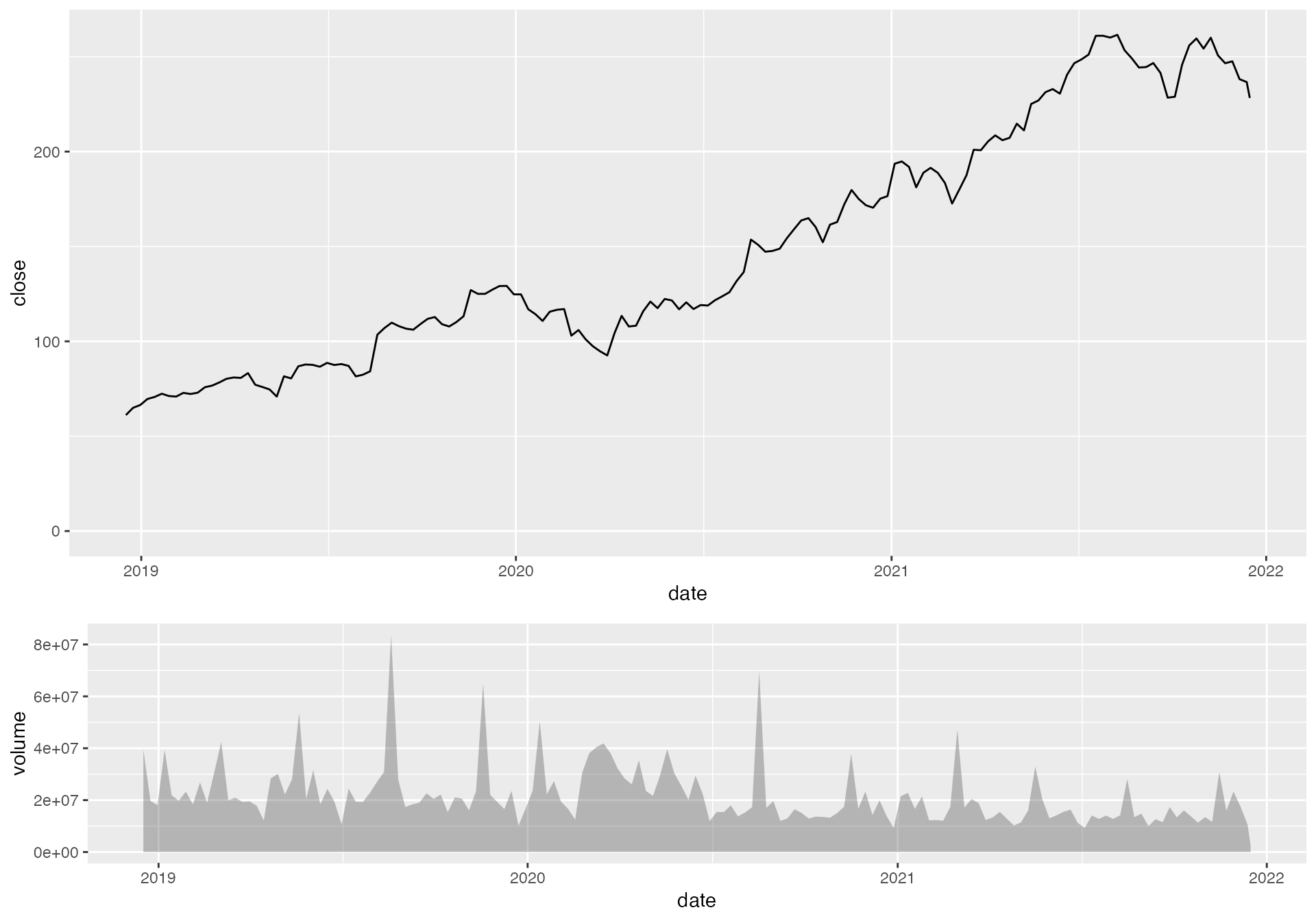
Fetch and plot historical prices.

history <- yahoo_history(ticker, interval = "1wk", days = 365 * 3)

p1 <- history %>% ggplot(aes(date, close)) + geom_line() + expand_limits(y = 0)
p2 <- history %>% ggplot(aes(date, volume)) + geom_area(alpha = 0.3) + expand_limits(y = 0)
ggarrange(p1, p2, nrow = 2, heights = c(2, 1))

Valuation

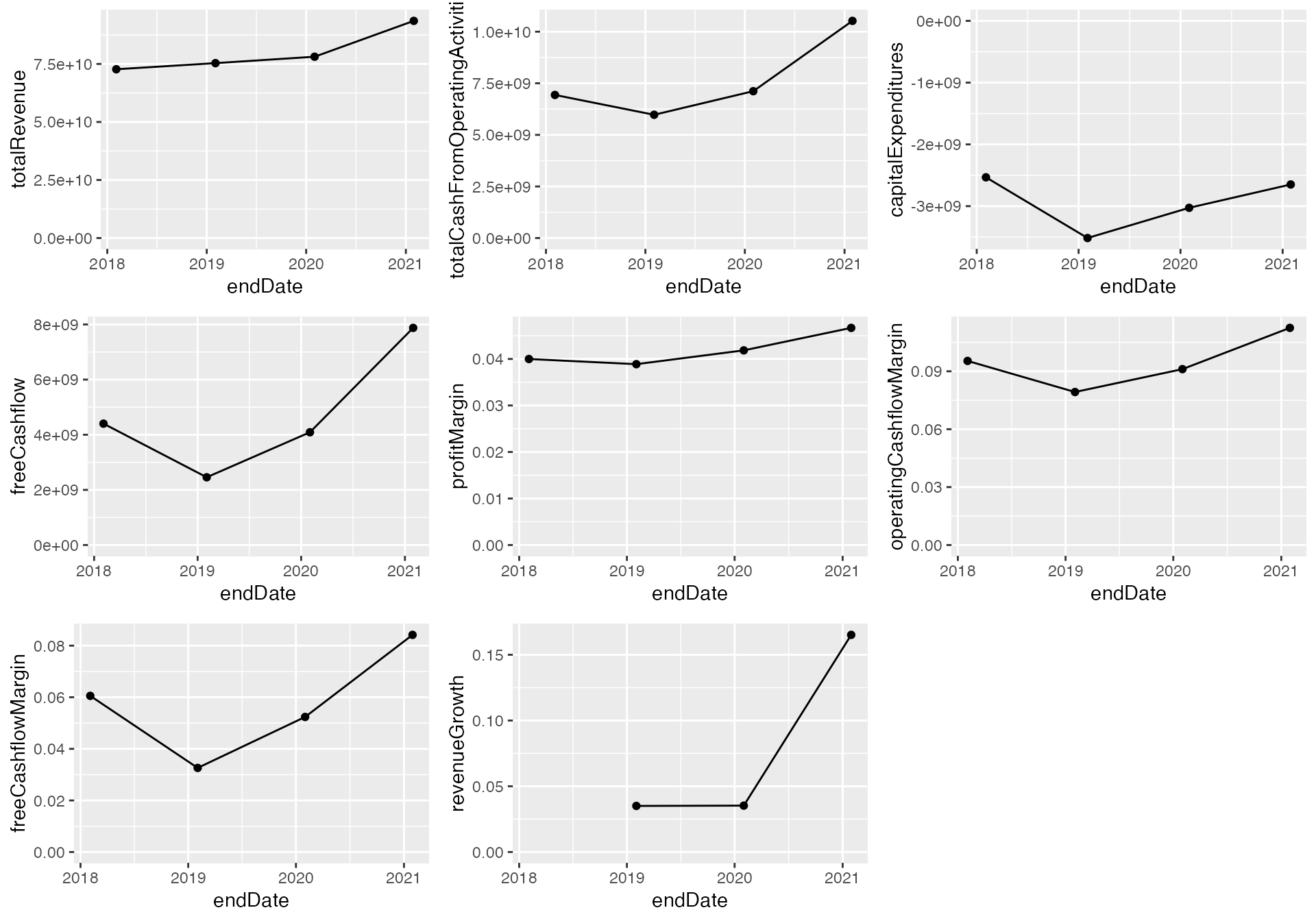
Fetch financials and calculate profit margin, operating cash flow margin, free cash flow margin, and revenue growth.

fin <- yahoo_financials(ticker) %>%
  arrange(endDate) %>%
  mutate(
    profitMargin = netIncomeFromContinuingOps / totalRevenue,
    operatingCashflowMargin = totalCashFromOperatingActivities / totalRevenue,
    freeCashflowMargin = freeCashflow / totalRevenue,
    revenueGrowth = (totalRevenue - lag(totalRevenue)) / totalRevenue
  )

p1 <- ggplot(fin, aes(endDate, totalRevenue)) + geom_point() + geom_line() + expand_limits(y = 0)
p2 <- ggplot(fin, aes(endDate, totalCashFromOperatingActivities)) + geom_point() + geom_line() + expand_limits(y = 0)
p3 <- ggplot(fin, aes(endDate, capitalExpenditures)) + geom_point() + geom_line() + expand_limits(y = 0)
p4 <- ggplot(fin, aes(endDate, freeCashflow)) + geom_point() + geom_line() + expand_limits(y = 0)
p5 <- ggplot(fin, aes(endDate, profitMargin)) + geom_point() + geom_line() + expand_limits(y = 0)
p6 <- ggplot(fin, aes(endDate, operatingCashflowMargin)) + geom_point() + geom_line() + expand_limits(y = 0)
p7 <- ggplot(fin, aes(endDate, freeCashflowMargin)) + geom_point() + geom_line() + expand_limits(y = 0)
p8 <- ggplot(fin, aes(endDate, revenueGrowth)) + geom_point() + geom_line() + expand_limits(y = 0)

ggarrange(p1, p2, p3, p4, p5, p6, p7, p8, ncol = 3, nrow = 3)

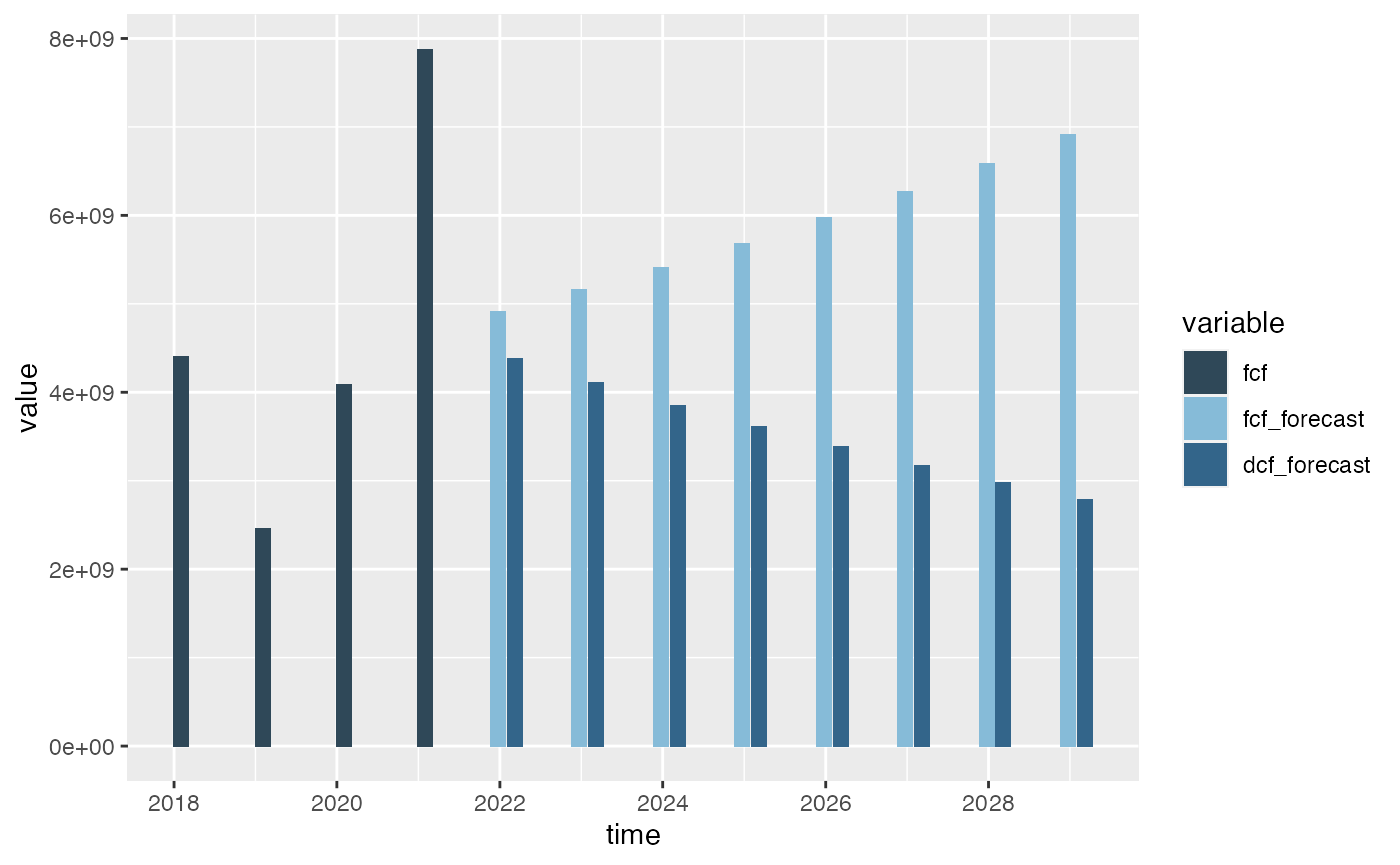
Now let’s take the last revenue value and apply revenue growth:

revenue_growth <- 0.05
freecashflow_margin <- 0.05
discount_rate <- 0.12
perpetuity_growth <- 0.02
t <- seq(1, 8)

time <- tail(fin$endDate, 1) + years(t)
base_revenue <- tail(fin$totalRevenue, 1)
fcf_forecast <- base_revenue * (1 + revenue_growth)^t * freecashflow_margin
dcf_forecast <- fcf_forecast / (1 + discount_rate)^t
terminal_value <- tail(fcf_forecast, 1) * (1 + revenue_growth) / (discount_rate - perpetuity_growth)

model <- data.frame(time, fcf_forecast, dcf_forecast) %>%
  melt(id.vars = 1) %>%
  bind_rows(fin %>% select(time = endDate, value = freeCashflow) %>% mutate(variable = "fcf")) %>%
  mutate(variable = factor(variable, levels = c("fcf", "fcf_forecast", "dcf_forecast"))) %>%
  as_tibble()

ggplot(model) +
  geom_bar(aes(x = time, y = value, fill = variable), stat = "identity", position = position_dodge2(preserve = "single"), width = as.numeric(days(150))) +
  scale_fill_manual(values = c("#2F4858", "#86BBD8", "#33658A"))

Calculate a net present value based on the discounted cash flow forecast, the terminal value, and shares outstanding:

tv <- terminal_value / summ$sharesOutstanding
npv <- sum(dcf_forecast) / summ$sharesOutstanding + tv

The calculated net present value is $210.53 of which $151.47 is terminal value.

Growth and profitability scenarios

To do.